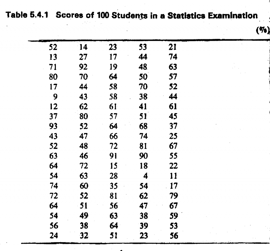
CONSTRUCTION OF A GROUPED FREQUENCY DISTRIBUTION
When we study large sets of data as in table below, our main objective is, first and foremost, to present the information in a more precise usable form. This is done by grouping our data into a number of – resulting in a grouped frequency distribution as we have in table below.
The format for constructing a grouped frequency table could be summarized as follows:
- decide on the number of classes into which the data are to be grouped;
- determine the clan width sometimes called the class interval;
- prepare the tally skeet;
- obtain the frequency table.
We shall illustrate the construction of a grouped frequency table by considering the following example.
Suppose we have data on the scores of a group of 100 students in a statistics examination as in Table above in order prepare a grouped frequency distribution for the data on scores, we flail first decide on the number of classes to create.
A formula exists for determining approximately the number of classes to form In constructing a grouped frequency table. It is known as Sturge’s rule, and is given as:
No. of groups = 1+ 3.322 log n
where n = the number of observed values. In our own case, n = too. Hence, by Sturge’s rule, the appropriate number of classes to create is approximately equal to
1 + 3.322 log 100 = 1 + 3.322 x 2
= 1 + 6.644
= 7.644 (approximately 8 groups)
This rule only gives a guide and does not provide a substitute for the sound judgement of the investigator in deciding on the number of classes. In fact, Sturge’s rule gives unreasonable result when n is very small or very large. A decision as to the appropriate number of classes to create is more or less a commonsense one and depends, among other things, on the nature of data, the range of. values covered, that is to say, the dispersion of the values, and of course on the total number of items being studied. For samples of about 30 to 50 observations, five to seven classes will be sufficient. For large temples of about 100 observations, we can create between 10 to 12 classes. For samples of up to 150 or more observations, we can have up to 15 classes. For very large samples, fewer than ten classes will generally result in much loss of information. For example, grouping the data in Table 5.4.1 on the scores of 100 students into three groups as follows: 0-40, 40-80, and over 80, would have been very unsatisfactory. Obviously, much information is lost.