RESPONSIBILITIES OF THE PRODUCTION MANAGER

Basically, the production manager is responsible for producing the goods in the required quantities and acceptable quality to meet the demand when it occurs. This must be done in the most economical way so as to maximize profit. In order to accomplish this, the production manager must be concerned with the following areas:

Production planning, production control, quality control, plant layout and materials handling, inventory control, work measurement, and wage incentive.

The above are the main problem areas in production management. In the following sections these are discussed in little detail.

1.         Production Planning

Production planning is the activity of forecasting the future demand for each product and translating this forecast to the requirements of inputs so that the products can be produced without any disruption to meet the demand.

Thus, production planning activity can be divided into two parts:

(i)         forecasting future demand for company products, and

(ii)        translating the demand of products to the demand it generates for various inputs, that is, determination of demand for various inputs.

(a)        Forecasting For Future Demand

Forecasts for demand can be obtained for (i) individual products or (ii) a group of products. If the number of products produced by the company is large, then it is more economical to group the products into a smaller number of groups according to some criteria such as their use, type etc. and forecast the demand for each group. Forecasts for individual products can be made either in quantity units or in monetary units but the group forecasts must be made in monetary units as the individual products in the group may be measured in different units such as tons, gallons, dozen etc. The individual forecasts in quantity units or in monetary units, or group forecasts in monetary units can be ob­tained by using different forecasting techniques such as collective opinion method; economic indicator method; time series analysis using regression or moving averages or exponential smoothing etc.

The forecast of demand obtained by using forecasting techniques is modified by a committee in the light of its knowledge of various factors such as planned advertising programmes, planned pricing policies, planned changes in competition etc. The modified forecast is taken to be the final forecast for demand.

The forecast for demand may be individual forecasts in quantity units (i.e. expressed in quantity units for individual products) in order to translate them to demand for inputs. This can be done for (i) individual forecasts and (ii) group forecasts as follows:

For individual products the forecast may be determined directly in quantity units. If the forecast is obtained in monetary units, dividing it by price per unit gives the forecast in quantity units.

Group forecast in monetary units can be converted to individual forecasts in quantity units as follows:

• Obtain the proportion of each individual product in the group from past sales records.
• Multiply the group forecast by the proportions obtained above. These give the forecast for individual products in the group in monetary units.
• Divide the individual monetary forecast obtained for each individual product by its price per unit quantity to obtain the individual forecast in quantity units.

(b)        Determination of demand for inputs

The demand for company products obtained by sales forecasting techniques can be translated to the demand it generates for various inputs as follows:

(i)         Obtain the demand for each individual product in quantity units.

(ii)        Obtain the quantity that must be produced, that is, production level of each product by making an allowance for defectives. If ‘d’ is the average fraction of defectives of production output of the product, then Production level =

Forecast for demand in quantity units (1 – d)

(iii)       Determine the requirement of inputs needed to produce a unit of the product. This can be done by using the operation sheet or routine sheet or bill of materials for the product which specifies the requirements of all inputs for a unit output of the product.

(iv)       Obtain the requirement of inputs for each individual product by multiplying the requirements of inputs for a unit of product obtained in (iii) by production level of that product obtained in (iii).

(v)        Construct an input demand schedule by adding the demand for each input createdby individual products. That is, for a given input and a time period, the respective demands generated by various products is totaled. This gives the total demand for that input for the time period concerned. This must be done for all the inputs, that is, materials, parts, machine times, labour etc.

The input demand schedule obtained in (v) gives the quantities of each input for each time period that must be on hand to meet the demand for products. The company can then make arrangements to procure these inputs in required quantity prior to the time they will actually be needed.

2.         Production Control

Production control deals with the efficient utili­zation of plant resources, that is, raw materials, parts, equipment and labour to produce the products in required quantity and quality in time to satisfy the demand. This can be accomplished only by exercising some control over the activities in the plant. Since a company usually produces a number of products, production control basically involves designing a schedule called operations schedule showing which activities (i.e. operations) must be carried out on which products at what time intervals. After an operation schedule is obtained, it must be effectively implemented. Progress of production must be checked periodically and corrective action must be ·taken if the actual progress of production deviates from the operation schedule.

Operations Schedule

As indicated above operations schedule is a time table for all the activities showing which operation must be done on which products at what time. To prepare an operation schedule it is necessary to obtain the following information for the planned period: number of products to be produced; quantity of each product andtime at which they are needed, inputs for the products; type of operations needed, operation time per unit of product for each operation, and sequence of operations for each product. This information is obtained in production planning. Using the above information an efficient schedule of operations is obtained by using different scheduling techniques.

Once an operations schedule is prepared for a period of time, it must be effectively implemented. Production control department can make periodic checks on the progress of production by obtaining reports of output of each operation. These can then be compared with the operations schedule to check for any deviations.

There will always be a difference between actual output and scheduled outputs for each operation. Ifthis difference is small nothing may be done and production is allowed to continue. If the difference between the scheduled and actual output is significant, corrective action must be taken so that the completion time of products is not delayed.

If an operation is ahead of schedule, then it may be allowed to continue or it may be slowed down to avoid high storage of its outputs between that operation and next operation. However, running ahead of schedule does not create much problems. If an operation is running behind schedule, the causes for it must be determined and appropriate corrective action must be taken. The causes may be material storage, frequent breakdown of machines, inefficiency of machine operators, improper use of machines etc. Also it may be necessary to have overtime, or extra shifts in order to make up for the lost output due to behind schedule operations.

The production manager is responsible for the effective control of all activities of the production department.

3.         Quality Control

One of the most important responsibilities of theproduction manager is to ensure that the output of the company products are of acceptable quality. The importance of this aspect of production needs no explanation as the reputation of company products largely depends on their quality.

In production, a set of inputs is converted into a set of outputs through a conversion process. Therefore, the quality of outputs depend on the quality of inputs and the different operations of the conversion process. Thus, the variations of the quality of outputs from the expected quality occur due to variations of the quality of inputs and variation of different operations of the conversion process. It is therefore clear that in order to control the quality of output it is necessary to control the quality of inputs and the operations of the conversion process.

Once a product is produced, its quality is determined and it may not be possible to change its quality. Therefore, it is the quality of future output that must be controlled.

Thus, quality control refers to controlling the quality offuture output by controlling the quality of inputs and the adjustments of equipment for various operations of the conversion process. It is more convenient to determine any changes in inputs or conversion process by checking the quality of output. Again, it is impossible to check the quality of each unit of output by inspection. Therefore, periodic samples from the output are taken and the quality of items in these samples are used as the basis for determining whether any change in, input or conversion process has taken place. This method is called “statistical quality control”. The objective of statistical quality control is to set up a formal control system on the output whereby changes of input of conversion process may be made known for necessary corrective action. There are two main control systems used in quality control namely (i) “control charts for variables” and (ii) “control charts for number of defectives” or “control charts for fraction of defectives”.

(a)        Control Chart for Variables

Control chart for variables is used in determining whether the process is in control (i.e., the quality of products are acceptable implying no apparent change in inputs or conversion process has occurred) or out of control (i.e., there seem to be some changes in inputs and/or conversion process) in situations in which the quality of the product is determined by a measurement of a characteristic of the product such as length, diameter, weight, percentage of an ingredient etc. The characteristic which determines the quality of the product is called the variable.

In order to control a variable, its average and dispersion must be controlled. This is done by a control chart for variables. Control charts for variables are represented by two charts called “control chart for averages of the variable” and “control chart for ranges”. The latter controls the dispersion of the variable.

If m is the expected average of the variable, and S2 is the variance of the variable for accep­table quality of product, then the control chart for averages gives two limits within which sample averages of the variable of periodic samples must lie if there is no reason to believe that there is any change in the average of the variable. If n is the size of the periodic sample then the averages of the samples must lie between  and where k is usually selected out of2, 2.5 and 3. These two values are called “lower control limit” and “upper control limit” for averages. Similarly, a control chart for ranges gives two limits within which the sample range must lie if the dispersion of the variable is unchanged. The two limits for ranges are given by (d₂s – kd₃s) and (d₂s + kd₃s) where d₂ and d₃ can be obtained from quality control tables for the sample size (n) used and k is 2 or 2.5 or 3. These two limits namely, (d₂s – kd₃s) and (d₂s + kd₃s) are called the “lower control limit for ranges” and “upper control limit forranges” respectively. Since the sample range cannot be negative, if the value of (d2 s – kd3 s) is negative then the lower control limit for ranges is taken to be zero. These control charts can be diagrammatically presented as follows:

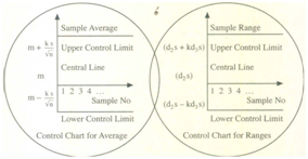
Fig. 1.0: Control Chart for Variables

In this case, samples of same size n are taken from the output periodically. For each item of the sample, the characteristic which determines the quality (i.e. variable) is measured accurately. The sample average of the variable and sample range of the variable are calculated using the measurements of the variable for items of the sample. For each sample, average of the variable and sample range of the variable are plotted on the control chart for averages and control chart for ranges. If both the points plotted in the two charts lie within the control limits then the process is assumed to be in control. Periodically, the samples are taken from the output and the procedure repeated. As long as the points plotted on the two charts lie between the control limits and an undue proportion of points such as seven consecutive points or out of 11 points or 12 out of 14 points or 14 out of 17, points do not fall on one side of the central line of either chart the process is assumed to be in control and production is continued. When a point falls outside the control limits of the chart or’ an undue proportion of points falls on one side of the central line, the process is assumed to be out of control, that is some change has taken place in inputs on the conversion process.

Production is stopped and investigation carried out to determine the changes that have occurred in the quality of inputs or conversion process and corrective action is taken.

(b) Control Charts for Defectives

Control charts for defectives are used when it is not convenient to use the control chart for variables. This happens if there are a number of characteristics which determine the quality, or accurate measurement of characteristics is uneconomical.

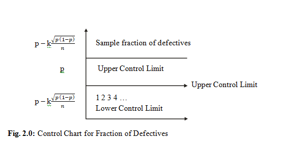
Here the change in the production process is determined by controlling the fraction of defectives in output. If the allowable fraction of defectives in the output is p and periodic samples of size n are taken, the fraction of defectives in the sample must lie between p – k and p + k if there is no apparent change of fraction of defectives in the output. Thus, p – k and p + k where k is 2, 2.5 or 3, are the “lower control limit for fraction of defectives” and “upper control limit for fraction of defectives.” This is shown in Figure 23.2.

Here the periodic samples of same size are taken and fraction of defectives in the samples determined and plotted on the control chart. As long as the points lie between the two control limits the process is assumed to be in control and production is continued. Once a point falls outside control limits, process is assumed to beout of control, an investigation is carried out to determine the causes for change and corrective action is taken.

4.         Plant Layout and Materials Handling

Plant layout is the activity of arranging different departments and equipment in the buildings of the factory plant for efficient operation of the system. It is mainly a responsibility of the Production Engineer rather than the Production Manager.

Plant layout consists of two main parts: (i) arrangement of production and service departments and (ii) arrangement of production facilities (i.e. equipment) of the production department, in the buildings of the factory. The goal is to develop an arrangement which will permit an efficient flow of work in terms of distance and cost.

The main purpose of a planned plant lay­out is:

(i)         to integrate the production centres of the plant into a logical, balanced and efficient production unit;

(ii)        to facilitate satisfactory movement of mate­rials and personnel, and to have an efficient control mechanism of such movement; (iii) to provide a logical distribution of the functional facilities in the plant;

(iv)       to ensure proper allocation and utilization of space to the production and service departments;

(v)        to provide convenience of operations for operation and supervision.

The main factors to be considered in layout planning in a manufacturing organization include the following:

(i)         Availability of space, physical characteristic of building, space requirements In production and service departments

(ii)        Types of products to be produced andtheir proportions such as physical state (solid, liquid or gas), weight, volume, durability, storage difficulties etc.

(iii)       Type of production system: that is, continuous or intermittent production system, and single flow or multi flows of materials

(iv)       Types of operations: types of machinery involved and their requirements etc.

(v)        Sequence of operations and its rigidity

(vi)       Types of inspection: centralized or decen­tralized inspection etc.

(vii)      Hazards: nature of risk due to moving parts of equipment, projecting equipment parts and suspended weights; air pollution; types of risks involved; precautionary measures that can be taken to ensure the safety of personnel and plant

(viii)     Adaptability to changes in products, product design, new products etc.

(ix)       Types of material handling system to be used.

4.         Materials Handling

This deals with the type of equipment used for transporting material between operations. There are many types of material handling equipment such as conveyors of different types, different industrial trucks and different type of cranes and hoists etc. The type or types selected for a plant depend on the following:

(i)         types of products to be produced and their physical proportions such as weight, volume, physical state etc.;

(ii)        required path of travel between operations; one path or number of paths;

(iii)       physical characteristics of building;

(iv)       required handling capacity depending on the output capacity of the production equipment;

(v)        cost aspect of materials handling equip­ment.

Design of plant layout and materials handlingsystem must be done concurrently as the two are interrelated. This is an activity usually done before starting production and may need some changes after starting production due to changes made in products after designing the system.

5.         Inventory Control

(a)        Need for Inventories:

The main reason for keeping inventories or stocks of an item is to satisfy demand for that item when it occurs. It is physically impossible and economically unsound to have goods arrive when the demand for them occurs. Items must be in stock (i.e., in inventory) to be used when the demand occurs. In manufacturing organizations, items kept in inventory include raw materials and parts, machine parts for equipment to carry out production without disruption, and finished products to cater for the demand when it occurs.

Other reason for keeping inventories include the following

(i)         To take advantage of seasonally fluctuating prices of the raw materials or parts. They can be purchased in large quantities when the prices are low and kept in inventory to be used when demand occurs.

(ii)        To take advantage of quantity discounts (or price discounts). When the price per unit changes with the quantity purchased, it may be economical to purchase in larger quantities at cheaper unit prices and keep in inventory to be used later.

(iii)       To level out the production schedule by keeping inventories of finished products produced in slack demand periods to cater for part of the demand in peak demand periods.

(iv)       To reduce ordering and handling cost. By ordering large quantities, the number of orders can be reduced thereby reducing the total ordering and handling cost that occurs whenever an order is made.

(b) Inventory Decision

The fundamental decision that must be.made in inventory control is “when to order,” and “how much to order”, such that total cost is minimized. Ordering too much increases cost of storage and opportunity cost of money tied up with the items. Ordering too little will result in shortages of items to fill the demand for them when it occurs. Ordering quantity must be determined to balance the cost of storage due to excessive inventory and cost of shortages due to insufficient inventory. This is done by’ considering the relevant costs and minimizing the total cost by formulating a mathematical model under reasonable assumptions.

(c) Terminology

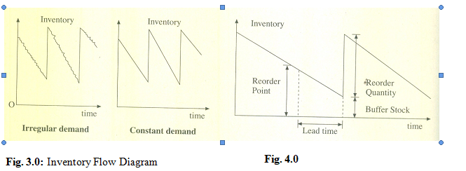
Inventory or stock of an item decreases with time according to the usage of the item (that is, demand pattern). When a new order is received the stock instantly increases by the quantity of item received. The general inventory – time diagram is given in Figure 23.3.

The following terminology is used in inventory control:

(i)         Procurement time or lead time: The time interval between the time at which the stocking point decides to make an order to replenishes the inventory and the time at which the order arrives and is ready foruse. This consists of administrative time for making the order, time to fill the order at the source, the transportation time and the inspection time at the receiving end. Lead time is estimated by estimating its components given above and is usually assumed to be constant for each order.

(ii)        Safety stock or buffer stock: This is the amount of inventory or stock kept to cater for any delay in delivery time or to satisfy any increased demand during lead time.

(iii)       Reorder point: Reorder point is the level of inventory at the time when a new order is made. Usually reorder point is determined in advance (by a mathematical calculation allowing for demand during lead time) and the inventory controller will make a new order whenever the inventory level falls to reorder point.

(iv)       Reorder quantity or lot size: This is the quantity of items ordered at a time.

These are illustrated in Figure 23.4.

(d) Relevant Costs

(i) Procurement Cost

This is the cost associated with the purchasing of items input and manufacturing of items for finished product.

Procurement cost has two components namely a fixed cost that is incurredwhenever an order is made (or production run is started), and a variable cost that depends on the quantity ordered or produced. Fixed cost may comprise administrative cost of processing the order, transportation cost (sometimes) and receiving cost. The variable cost may consist of purchase cost (or production cost), transportation cost (most cases), receiving and inspection cost. Procurement cost can be expressed in the form Cp = K + c Q where K is the ‘fixed cost, c is the variable cost per unit and Q is the quantity ordered. Value of K and c can be estimated by estimating their components.

(ii) Inventory Carrying Cost

This is the cost of storage and may consist of warehouse rental cost, cost of operating warehouse, breakage and pilferage in storage, insurance cost, opportunity cost etc.

Clearly, inventory holding cost depends on the inventory level and time period for which inventory is kept (carried)” The inventory holding-cost can be expressed as,

C_H = hx (average inventory) x (Total time inventory is carried)

Where, h is the inventory cost for unit per unit time, that is, the cost of keeping one unit in storage for a unit, and is estimated by estimating its components.

(iii) Shortage Cost:

This is the cost due to shortages and may arise due to unfilled demand or lost sales (or lost production time).

Clearly, like inventory carrying cost, shortage cost also depends on the shortage quantity and the time period for which shortages continue.

Shortage cost can be expressed as

CS = s x (average shortage) x (time period shortages occur)

Total cost of ordering Q units, is given by the sum of the above costs, that is, TC = C_P + C_H + C_S

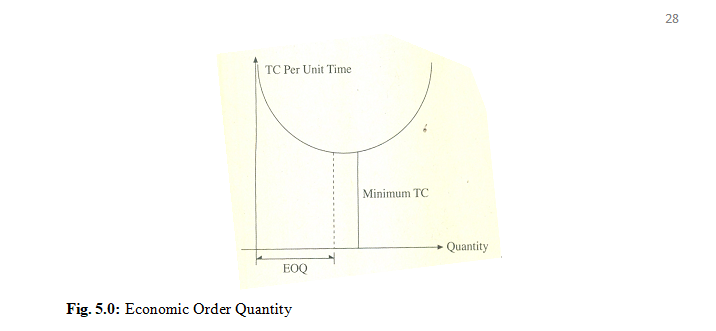
(e) Economic Order Quantity (EOQ)

It can be seen that the total cost per unit time decreases as the reorder quantity is increased, attains a minimum and then increases as the reorder quantity increases as shown in Figure 23.5.

The quantity which gives the minimum total cost per unit time, is the most economical reorder quantity and is called the economic order quantity or EOQ. Economic order quantity is obtained by mathematical models for different inventory situations, under different assumptions. The basic economic order quantity (EOQ) formula is given by

EOQ = Q* =

And Minimum Total cost per unit time =

TC* =

Where Q* = Economic order quality (EOQ)

            K = fixed cost

D         =          demand per unit time

H         =          inventory carrying cost per unit time

TC       =          total cost per unit time

C         =          variable cost per unit

EOQ is obtained under the following assumptions:

*          The demand or consumption rate of the item is constant. That is, items are assumed to be withdrawn from the inventory at a constant rate of D per unit time.

*          The items are ordered in lot sizes of the same quantity – Q* (i.e. EOQ) and the entire lot ordered is delivered at one time.

*          The lead time is known in advance and is constant.

*          No buffer stock and no shortages. That is, the minimum inventory level is zero.

The production manager is responsible for developing efficient inventory policies for inputs, (i.e., raw materials, parts, machine parts etc.) and for finished products, and implementing them.

6.         Wage Incentive Schemes

Wage incentive schemes are designed to increase the productivity of employees through rewarding them by paying a bonus, that is, a financial incentive for increased productivity.

There are a number of different wage incentive schemes. The common characteristics of all wage incentive schemes are that:

(i)         All plans are based on some standard of performance i.e., out-put, which is usually obtained by work measurement procedures, that company has the right to expect from the employees.

(ii)        All plans have a percentage point of the standard performance at which the incentives start. That is, for example, for productivity over 80% of the standard performance, the company may pay a reward, usually a percentage of pay. Here, the wage incentives start at 80% of standardperformance.

(iii)       All plans have a predetermined manner in which incentives are determined for performance over the required percentage point of performance. For example, for each additional percentage of productivity (i.e. output) the company may pay one percent of the wage.

The following are some of the commonly used wage incentive plan:

(i)         Full participation plan beginning at 100% efficiency. That is, incentives start at 100% efficiency (i.e. at standard performance or output) and the earning is increased by one percent for each one percent increase of output beyond 100%. That is, the incentive is 1 % of base salary for each 1 % increase of output above 100%.

(ii)        Less than full participation plan beginning at 100% efficiency. Here the incentive starts at 100% efficiency but the incentive is less than 1 % (say 2/3%) of the base salary for each 1% increase of output above 100%. This type of plan is used if the productivity of the employees without an incentive scheme is closer to standard performance.

(iii)       Full participation plan beginning at less than 100% efficiency. Here the incentive starts at a point of productivity less than the standard performance (say 80% of standard performance) and the incentive is 1% of base salary for each 1% increase of output beyond the percentage point at which incentives begin. This type of plan is usually used if the performance of employee before starting the incentive scheme is much more than standard performance expected. If theincentives begin at 100% efficiency, the productivity of the employee must be first increased to 100% without any additional earning before getting any incentive at all. Employees may think that the incentive is not worth the effort they will have to put, when the incentives begin at a lower point than 100%. With little more effort, they may be able to reach the performance at which incentives start and begin to receive incentive for increased performance.

(iv)       The step plan: Here the incentives start at either 100% efficiency, that is, at standard output or at a lower percentage of efficiency predetermined by the management. For efficiencies above this level, the hourly rate of pay is determined by Hourly rate of pay (C) x (efficiency) x (base rate per hour) where C is a constant predetermined by the management. Usually C is greater than 1. In this plan, the hourly rate has a sudden jump or step at the level of efficiency that the incentive starts. Therefore it is called the step plan. This plan is usually used in situations where the productivity is far below the standard performance level. The sudden jump of pay rate at the standard performance level or at the percentage point of efficiency motivates employees to attain at least that level of productivity so that they can increase the rate of their earnings.

Determination of the type of incentive plan to adopt depends on the company situation, performance level etc. It is the responsibility of the production manager to assess the performance levels of employees and if necessary to install an appropriate wage incentive plan to increase the productivity of the employees.

CONCLUSION

In this chapter we have attempted to discuss basic features of production management by examiningthe responsibilities of a production manager. Discussions are kept non-mathematical and brief. However, an attempt is made to highlight the essential facts in each section. Quantitative approaches to production management, that is, mathematical models and techniques, are not discussed here. The interested reader is referred to more specialised texts.